
K-MOOC 3주차 SVM의 이해와 활용
3주차 1차시
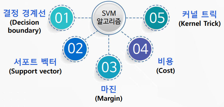
SVM의 이해와 활용

 서포트 벡터는 여러개가 가능

사이킷런의 그리드 서치(gridsearch)를 사용하여 간편하게 최적의 비용과 감마를 알아내기
# 패키지 및 데이터셋 추가
# GridSearchCV 는 최적의 조합을 만들어서 최고의 성능을 내는 것을 찾아줌
from sklearn.model_selection import GridSearchCV
from sklearn.metrics import classification_report
from sklearn.metrics import accuracy_score
from sklearn.model_selection import train_test_split
from sklearn.svm import SVC
import numpy as np
import pandas as pd

df = pd.read_csv("https://raw.githubusercontent.com/wikibook/machine-learning/2.0/data/csv/basketball_stat.csv")
train, test = train_test_split(df, test_size=0.2)
# 최적의 SVM 파라미터 찾기
# svm_parameters의 값들의 조합중 GridSearcgCV를 통해서 최적을 찾는다
def svc_param_selection(X, y, nfolds):
    svm_parameters = [{'kernel': ['rbf'],
                     'gamma': [0.00001, 0.0001, 0.001, 0.01, 0.1, 1],
                     'C': [0.01, 0.1, 1, 10, 100, 1000]}]
    clf = GridSearchCV(SVC(), svm_parameters, cv=nfolds)
    clf.fit(X, y)
    print(clf.best_params_)
    return clf

X_train = train[['3P', 'BLK']]
y_train = train[['Pos']]
clf = svc_param_selection(X_train, y_train.values.ravel(), 10)
{'C': 0.01, 'gamma': 1e-05, 'kernel': 'rbf'}
# 그리드 서치를 통해 얻은 C와 감마를 사용해 학습된 모델 테스트
X_test = test[['3P', 'BLK']]
y_test = test[['Pos']]

y_true, y_pred = y_test, clf.predict(X_test)

print(classification_report(y_true, y_pred))
print()
print("accuracy : "+ str(accuracy_score(y_true, y_pred)) )
              precision    recall  f1-score   support

           C       0.89      0.80      0.84        10
          SG       0.82      0.90      0.86        10

    accuracy                           0.85        20
   macro avg       0.85      0.85      0.85        20
weighted avg       0.85      0.85      0.85        20


accuracy : 0.85
comparison = pd.DataFrame({'prediction': y_pred,
                           'ground_truth': y_true.values.ravel()})
comparison
| prediction | ground_truth | |
|---|---|---|
| 0 | C | C |
| 1 | SG | SG |
| 2 | C | C |
| 3 | C | C |
| 4 | SG | SG |
| 5 | C | SG |
| 6 | C | C |
| 7 | SG | C |
| 8 | SG | C |
| 9 | SG | SG |
| 10 | SG | SG |
| 11 | SG | SG |
| 12 | SG | SG |
| 13 | SG | SG |
| 14 | C | C |
| 15 | C | C |
| 16 | SG | SG |
| 17 | SG | SG |
| 18 | C | C |
| 19 | C | C |
3주차 2차시
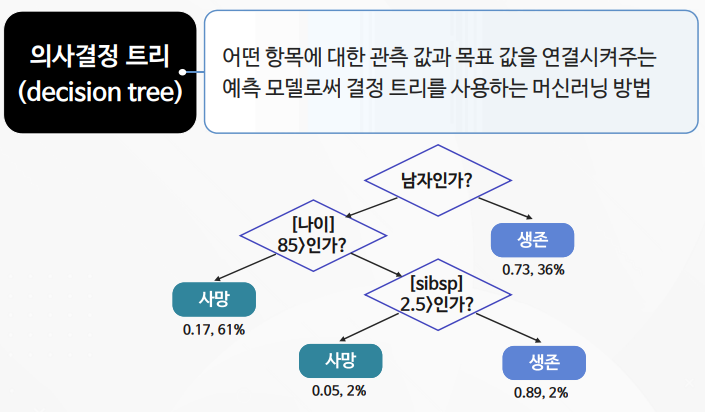
의사결정 트리의 이해 및 활용
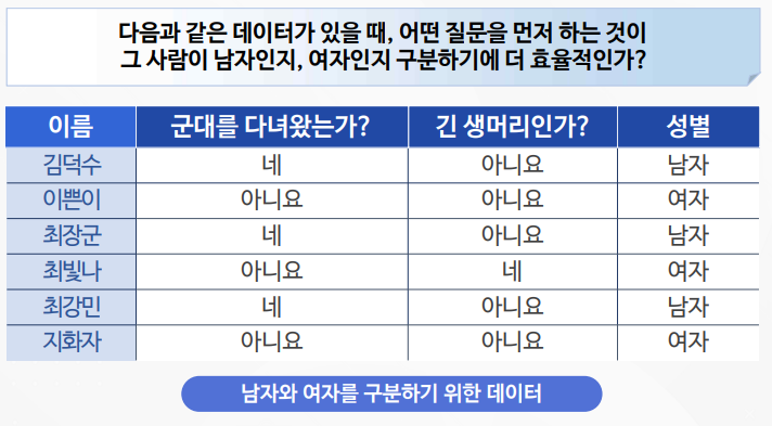
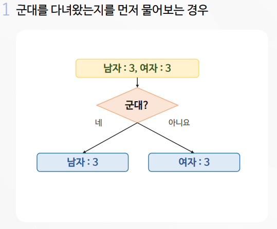
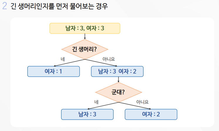
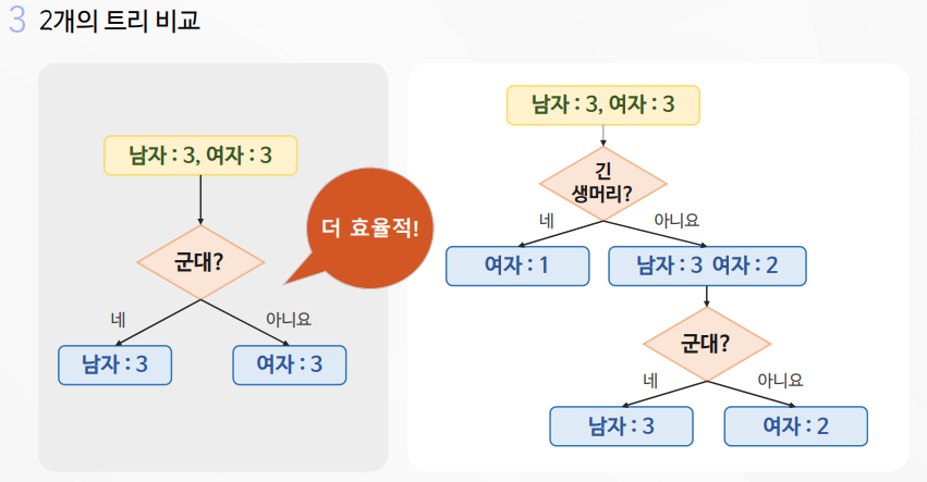


의사결정트리 실습
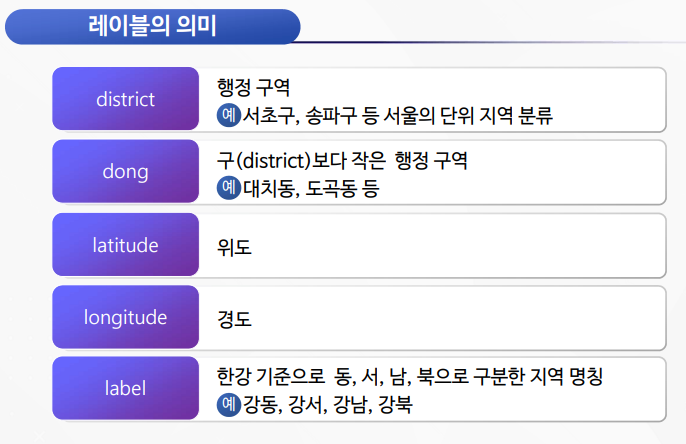
# 서울의 지역(구) 위치 데이터
import pandas as pd

district_dict_list = [
            {'district': 'Gangseo-gu', 'latitude': 37.551000, 'longitude': 126.849500, 'label':'Gangseo'},
            {'district': 'Yangcheon-gu', 'latitude': 37.52424, 'longitude': 126.855396, 'label':'Gangseo'},
            {'district': 'Guro-gu', 'latitude': 37.4954, 'longitude': 126.8874, 'label':'Gangseo'},
            {'district': 'Geumcheon-gu', 'latitude': 37.4519, 'longitude': 126.9020, 'label':'Gangseo'},
            {'district': 'Mapo-gu', 'latitude': 37.560229, 'longitude': 126.908728, 'label':'Gangseo'},

            {'district': 'Gwanak-gu', 'latitude': 37.487517, 'longitude': 126.915065, 'label':'Gangnam'},
            {'district': 'Dongjak-gu', 'latitude': 37.5124, 'longitude': 126.9393, 'label':'Gangnam'},
            {'district': 'Seocho-gu', 'latitude': 37.4837, 'longitude': 127.0324, 'label':'Gangnam'},
            {'district': 'Gangnam-gu', 'latitude': 37.5172, 'longitude': 127.0473, 'label':'Gangnam'},
            {'district': 'Songpa-gu', 'latitude': 37.503510, 'longitude': 127.117898, 'label':'Gangnam'},

            {'district': 'Yongsan-gu', 'latitude': 37.532561, 'longitude': 127.008605, 'label':'Gangbuk'},
            {'district': 'Jongro-gu', 'latitude': 37.5730, 'longitude': 126.9794, 'label':'Gangbuk'},
            {'district': 'Seongbuk-gu', 'latitude': 37.603979, 'longitude': 127.056344, 'label':'Gangbuk'},
            {'district': 'Nowon-gu', 'latitude': 37.6542, 'longitude': 127.0568, 'label':'Gangbuk'},
            {'district': 'Dobong-gu', 'latitude': 37.6688, 'longitude': 127.0471, 'label':'Gangbuk'},

            {'district': 'Seongdong-gu', 'latitude': 37.557340, 'longitude': 127.041667, 'label':'Gangdong'},
            {'district': 'Dongdaemun-gu', 'latitude': 37.575759, 'longitude': 127.025288, 'label':'Gangdong'},
            {'district': 'Gwangjin-gu', 'latitude': 37.557562, 'longitude': 127.083467, 'label':'Gangdong'},
            {'district': 'Gangdong-gu', 'latitude': 37.554194, 'longitude': 127.151405, 'label':'Gangdong'},
            {'district': 'Jungrang-gu', 'latitude': 37.593684, 'longitude': 127.090384, 'label':'Gangdong'}
         ]

train_df = pd.DataFrame(district_dict_list)
train_df = train_df[['district', 'longitude', 'latitude', 'label']]
# 서울의 대표적인 동 위치 데이터
dong_dict_list = [
            {'dong': 'Gaebong-dong', 'latitude': 37.489853, 'longitude': 126.854547, 'label':'Gangseo'},
            {'dong': 'Gochuk-dong', 'latitude': 37.501394, 'longitude': 126.859245, 'label':'Gangseo'},
            {'dong': 'Hwagok-dong', 'latitude': 37.537759, 'longitude': 126.847951, 'label':'Gangseo'},
            {'dong': 'Banghwa-dong', 'latitude': 37.575817, 'longitude': 126.815719, 'label':'Gangseo'},
            {'dong': 'Sangam-dong', 'latitude': 37.577039, 'longitude': 126.891620, 'label':'Gangseo'},

            {'dong': 'Nonhyun-dong', 'latitude': 37.508838, 'longitude': 127.030720, 'label':'Gangnam'},
            {'dong': 'Daechi-dong', 'latitude': 37.501163, 'longitude': 127.057193, 'label':'Gangnam'},
            {'dong': 'Seocho-dong', 'latitude': 37.486401, 'longitude': 127.018281, 'label':'Gangnam'},
            {'dong': 'Bangbae-dong', 'latitude': 37.483279, 'longitude': 126.988194, 'label':'Gangnam'},
            {'dong': 'Dogok-dong', 'latitude': 37.492896, 'longitude': 127.043159, 'label':'Gangnam'},

            {'dong': 'Pyoungchang-dong', 'latitude': 37.612129, 'longitude': 126.975724, 'label':'Gangbuk'},
            {'dong': 'Sungbuk-dong', 'latitude': 37.597916, 'longitude': 126.998067, 'label':'Gangbuk'},
            {'dong': 'Ssangmoon-dong', 'latitude': 37.648094, 'longitude': 127.030421, 'label':'Gangbuk'},
            {'dong': 'Ui-dong', 'latitude': 37.648446, 'longitude': 127.011396, 'label':'Gangbuk'},
            {'dong': 'Samcheong-dong', 'latitude': 37.591109, 'longitude': 126.980488, 'label':'Gangbuk'},

            {'dong': 'Hwayang-dong', 'latitude': 37.544234, 'longitude': 127.071648, 'label':'Gangdong'},
            {'dong': 'Gui-dong', 'latitude': 37.543757, 'longitude': 127.086803, 'label':'Gangdong'},
            {'dong': 'Neung-dong', 'latitude': 37.553102, 'longitude': 127.080248, 'label':'Gangdong'},
            {'dong': 'Amsa-dong', 'latitude': 37.552370, 'longitude': 127.127124, 'label':'Gangdong'},
            {'dong': 'Chunho-dong', 'latitude': 37.547436, 'longitude': 127.137382, 'label':'Gangdong'}
         ]

test_df = pd.DataFrame(dong_dict_list)
test_df = test_df[['dong', 'longitude', 'latitude', 'label']]
train_df.head()
| district | longitude | latitude | label | |
|---|---|---|---|---|
| 0 | Gangseo-gu | 126.849500 | 37.551000 | Gangseo |
| 1 | Yangcheon-gu | 126.855396 | 37.524240 | Gangseo |
| 2 | Guro-gu | 126.887400 | 37.495400 | Gangseo |
| 3 | Geumcheon-gu | 126.902000 | 37.451900 | Gangseo |
| 4 | Mapo-gu | 126.908728 | 37.560229 | Gangseo |
test_df.head()
| dong | longitude | latitude | label | |
|---|---|---|---|---|
| 0 | Gaebong-dong | 126.854547 | 37.489853 | Gangseo |
| 1 | Gochuk-dong | 126.859245 | 37.501394 | Gangseo |
| 2 | Hwagok-dong | 126.847951 | 37.537759 | Gangseo |
| 3 | Banghwa-dong | 126.815719 | 37.575817 | Gangseo |
| 4 | Sangam-dong | 126.891620 | 37.577039 | Gangseo |
# 학습 및 테스트에 불필요한 특징 제거
train_df.drop(['district'], axis=1, inplace = True)
test_df.drop(['dong'], axis=1, inplace = True)

X_train = train_df[['longitude', 'latitude']]
y_train = train_df[['label']]

X_test = test_df[['longitude', 'latitude']]
y_test = test_df[['label']]
from sklearn import tree
import numpy as np
import matplotlib.pyplot as plt
from sklearn import preprocessing
def display_decision_surface(clf,X, y):

    x_min = X.longitude.min() - 0.01
    x_max = X.longitude.max() + 0.01
    y_min = X.latitude.min() - 0.01
    y_max = X.latitude.max() + 0.01

    n_classes = len(le.classes_)
    plot_colors = "rywb"
    plot_step = 0.001

    xx, yy = np.meshgrid(np.arange(x_min, x_max, plot_step),
                        np.arange(y_min, y_max, plot_step))

    Z = clf.predict(np.c_[xx.ravel(), yy.ravel()])
    Z = Z.reshape(xx.shape)
    cs = plt.contourf(xx, yy, Z, cmap=plt.cm.RdYlBu)

    for i, color in zip(range(n_classes), plot_colors):
        idx = np.where(y == i)
        plt.scatter(X.loc[idx].longitude,
                    X.loc[idx].latitude,
                    c=color,
                    label=le.classes_[i],
                    cmap=plt.cm.RdYlBu, edgecolor='black', s=200)


    plt.title("Decision surface of a decision tree",fontsize=16)
    plt.legend(bbox_to_anchor=(1.05, 1), loc=2, borderaxespad=0., fontsize=14)
    plt.xlabel('longitude',fontsize=16)
    plt.ylabel('latitude',fontsize=16)
    plt.rcParams["figure.figsize"] = [7,5]
    plt.rcParams["font.size"] = 14
    plt.rcParams["xtick.labelsize"] = 14
    plt.rcParams["ytick.labelsize"] = 14
    plt.show()
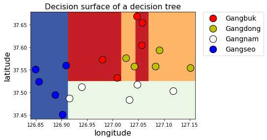
# 파라미터 없이 학습
le = preprocessing.LabelEncoder()
y_encoded = le.fit_transform(y_train)

clf = tree.DecisionTreeClassifier(random_state=35).fit(X_train, y_encoded)
display_decision_surface(clf, X_train, y_encoded)
C:\Users\Administrator\.conda\envs\venv\lib\site-packages\sklearn\utils\validation.py:63: DataConversionWarning: A column-vector y was passed when a 1d array was expected. Please change the shape of y to (n_samples, ), for example using ravel().
  return f(*args, **kwargs)
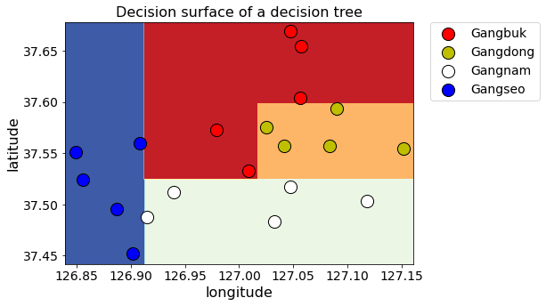
# 파라미터를 설정한 모델 시각화
clf = tree.DecisionTreeClassifier(max_depth=4,
                                  min_samples_split=2,
                                  min_samples_leaf=2,
                                  random_state=70).fit(X_train, y_encoded.ravel())
display_decision_surface(clf,X_train, y_encoded)
from sklearn.metrics import accuracy_score
pred = clf.predict(X_test)

print("accuracy : " + str( accuracy_score(y_test.values.ravel(),
                                          le.classes_[pred])) )
comparison = pd.DataFrame({'prediction':le.classes_[pred],
                           'ground_truth':y_test.values.ravel()})
comparison
accuracy : 1.0
| prediction | ground_truth | |
|---|---|---|
| 0 | Gangseo | Gangseo |
| 1 | Gangseo | Gangseo |
| 2 | Gangseo | Gangseo |
| 3 | Gangseo | Gangseo |
| 4 | Gangseo | Gangseo |
| 5 | Gangnam | Gangnam |
| 6 | Gangnam | Gangnam |
| 7 | Gangnam | Gangnam |
| 8 | Gangnam | Gangnam |
| 9 | Gangnam | Gangnam |
| 10 | Gangbuk | Gangbuk |
| 11 | Gangbuk | Gangbuk |
| 12 | Gangbuk | Gangbuk |
| 13 | Gangbuk | Gangbuk |
| 14 | Gangbuk | Gangbuk |
| 15 | Gangdong | Gangdong |
| 16 | Gangdong | Gangdong |
| 17 | Gangdong | Gangdong |
| 18 | Gangdong | Gangdong |
| 19 | Gangdong | Gangdong |
3주차 3차시
나이브 베이즈의 이해 및 활용

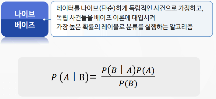
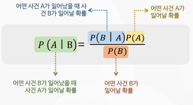
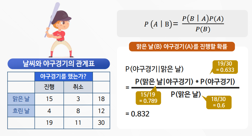
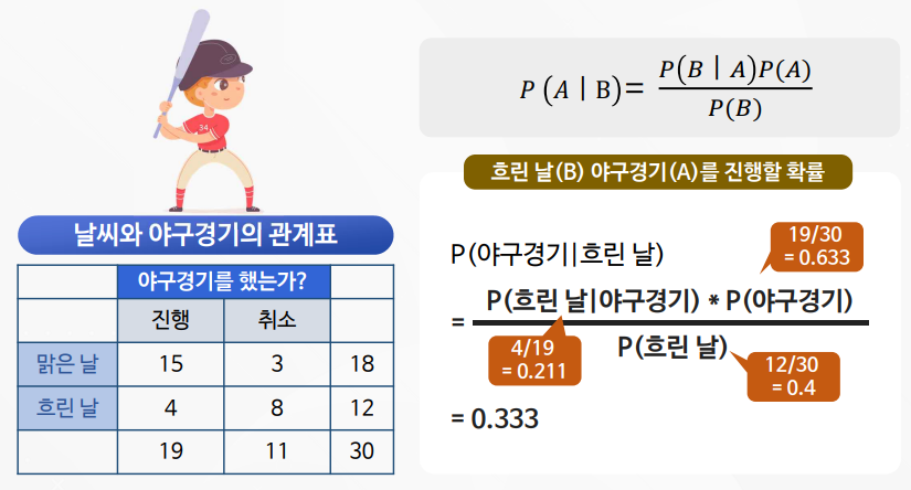


나이브 베이즈 실습
import pandas as pd
from sklearn.datasets import load_iris
from sklearn.model_selection import train_test_split
from sklearn.naive_bayes import GaussianNB
from sklearn import metrics
from sklearn.metrics import accuracy_score
# 데이터 획득 및 탐색
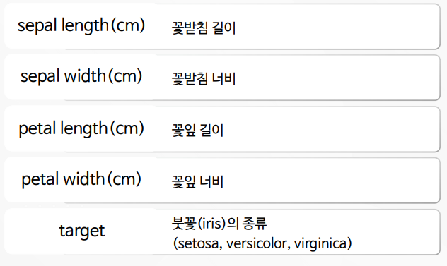
dataset = load_iris()
df = pd.DataFrame(dataset.data, columns=dataset.feature_names)
df['target'] = dataset.target
df.target = df.target.map({0:"setosa", 1:"versicolor", 2:"virginica"})
df.head()
| sepal length (cm) | sepal width (cm) | petal length (cm) | petal width (cm) | target | |
|---|---|---|---|---|---|
| 0 | 5.1 | 3.5 | 1.4 | 0.2 | setosa |
| 1 | 4.9 | 3.0 | 1.4 | 0.2 | setosa |
| 2 | 4.7 | 3.2 | 1.3 | 0.2 | setosa |
| 3 | 4.6 | 3.1 | 1.5 | 0.2 | setosa |
| 4 | 5.0 | 3.6 | 1.4 | 0.2 | setosa |
df.target.value_counts()
virginica     50
versicolor    50
setosa        50
Name: target, dtype: int64
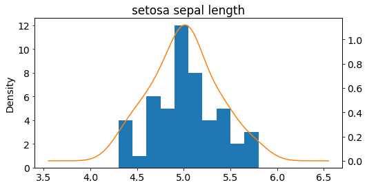
# 데이터 시각화
setosa_df = df[df.target == "setosa"]
versicolor_df = df[df.target == "versicolor"]
virginica_df = df[df.target == "virginica"]
ax = setosa_df['sepal length (cm)'].plot(kind='hist')
setosa_df['sepal length (cm)'].plot(kind='kde',
                                    ax=ax,
                                    secondary_y=True,
                                    title="setosa sepal length",
                                    figsize = (8,4))
<AxesSubplot:label='320b5d70-c443-40ae-9ccb-5a32cdd55cf1'>
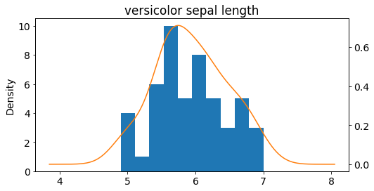
ax = versicolor_df['sepal length (cm)'].plot(kind='hist')
versicolor_df['sepal length (cm)'].plot(kind='kde',
                                        ax=ax,
                                        secondary_y=True,
                                        title="versicolor sepal length",
                                        figsize = (8,4))
<AxesSubplot:label='72428b9d-1ff2-41bd-b5ee-c933d4dc0602'>
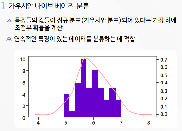
# 가우시안 나이브 베이즈 분류
X_train,X_test,y_train,y_test=train_test_split(dataset.data,
                                               dataset.target,test_size=0.2)
model = GaussianNB()
model.fit(X_train, y_train)

expected = y_test
predicted = model.predict(X_test)
print(metrics.classification_report(y_test, predicted))
print(accuracy_score(y_test, predicted))
              precision    recall  f1-score   support

           0       1.00      1.00      1.00         7
           1       1.00      1.00      1.00        11
           2       1.00      1.00      1.00        12

    accuracy                           1.00        30
   macro avg       1.00      1.00      1.00        30
weighted avg       1.00      1.00      1.00        30

1.0
# 혼동 행렬 확인
print(metrics.confusion_matrix(expected, predicted))
[[ 7  0  0]
 [ 0 11  0]
 [ 0  0 12]]
Leave a comment